class: center, middle # Atmospheric Boundary Layer turbulence theory ## Ashwin Vishnu Mohanan <img src="https://cdn.jsdelivr.net/gh/ashwinvis/talks@3ebeb930f997b97dfcf87ce65fc5253a74eb9735/./images/dp_eturb.svg" style="height: 5em;"/> ### [exabl.github.io/eturb](https://exabl.github.io/eturb) <img src="https://cdn.jsdelivr.net/gh/ashwinvis/talks@3ebeb930f997b97dfcf87ce65fc5253a74eb9735/./images/dp_su.gif" style="height: 3em;"/> <img src="https://cdn.jsdelivr.net/gh/ashwinvis/talks@3ebeb930f997b97dfcf87ce65fc5253a74eb9735/./images/dp_kth.svg" style="height: 3em;"/> <div style="font-size: 0.8em;"> <a rel="license" href="http://creativecommons.org/licenses/by/4.0/"><img alt="Creative Commons License" style="border-width:0; height: 1em;" src="https://i.creativecommons.org/l/by/4.0/88x31.png" /></a> All text in this presentation is licensed under a <a rel="license" href="http://creativecommons.org/licenses/by/4.0/">Creative Commons Attribution 4.0 International License</a>. Images and screenshots are copyright material. </div> ??? - Good morning all! - Now I will present my talk titled ... - Thank: SU for the opportunity to come here --- layout: false # Overview .left-column[ ## References ## Turbulence fundamentals ] .right-column[ - Essential quantities: \\( \tau,\,u_* \\) - Regions inside the boundary layer - Log-law of the wall - Effect of roughness ] --- # Overview .left-column[ ## References ## Turbulence fundamentals ## Monin-Obukhov similarity theory ] .right-column[ - Derivation using Buckingham Pi theorem - Physical meaning - Moeng's boundary condition variant ] --- # Overview .left-column[ ## References ## Turbulence fundamentals ## Monin-Obukhov similarity theory ## Possible compressible formulation ] .right-column[ - "Buoyancy term" - Expression for stability parameter, \\( N \\) ] --- # Overview .left-column[ ## References ## Turbulence fundamentals ## Monin-Obukhov similarity theory ## Possible compressible formulation ## Appendix: project update ] .right-column[ - Filtering - Next steps? ] --- # References 1. Pope, S.B. Turbulent Flows. Cambridge University Press, 2000. 1. Wyngaard, John C. Turbulence in the Atmosphere. Cambridge: Cambridge University Press, 2010. https://doi.org/10.1017/CBO9780511840524. 1. Monin, A S, and A M Obukhov. “Basic Laws of Turbulent Mixing in the Surface Layer of the Atmosphere,” 1954, 30. 1. Moeng, Chin-Hoh. “A Large-Eddy-Simulation Model for the Study of Planetary Boundary-Layer Turbulence.” Journal of the Atmospheric Sciences 41, no. 13 (July 1, 1984): 2052–62. https://doi.org/10.1175/1520-0469(1984)041<2052:ALESMF>2.0.CO;2. 1. Cushman-Roisin, Benoit, and Jean-Marie Beckers. “Stratification.” In International Geophysics, 101:347–64. Elsevier, 2011. https://doi.org/10.1016/B978-0-12-088759-0.00011-0. 1. Svensson, Gunilla, and Albert A. M. Holtslag. “Analysis of Model Results for the Turning of the Wind and Related Momentum Fluxes in the Stable Boundary Layer.” Boundary-Layer Meteorology 132, no. 2 (August 2009): 261–77. https://doi.org/10.1007/s10546-009-9395-1. 1. Maronga, Björn, Christoph Knigge, and Siegfried Raasch. “An Improved Surface Boundary Condition for Large-Eddy Simulations Based on Monin–Obukhov Similarity Theory: Evaluation and Consequences for Grid Convergence in Neutral and Stable Conditions.” Boundary-Layer Meteorology, October 29, 2019. https://doi.org/10.1007/s10546-019-00485-w. --- class: center, middle, inverse # Turbulence fundamentals --- layout: false ## Essential quantities ### Wall shear stress \\( \tau \\) and friction velocity \\( u_* \\) .pull-left[ Shear stress can be driven by: - molecular diffusion \\[ \tau_{ij} = \mu \frac{\partial u_i}{\partial x_j} \\] ... Newton's law of viscosity - turbulent diffusion \\[ \tau_{ij} = -\rho \overline{u_iu_j } \\] ... Reynolds stress tensor (statistical quantity) Friction velocity \\[ u_* = \sqrt{\frac{\tau}{\rho}} \\] ] .pull-right[ 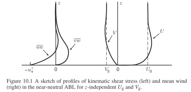 ] --- ## Observations from DNS of channel flows .pull-left[ N.B: \\( y \\) is the wall normal direction in engineering \\[ \delta_v = \text{viscous length scale},\quad \delta = \text{displacement thickness} \\] \\[ u^+ = \bar{U} / u_* , \quad y^+ = y / \delta_v \\]  ] .pull-right[ 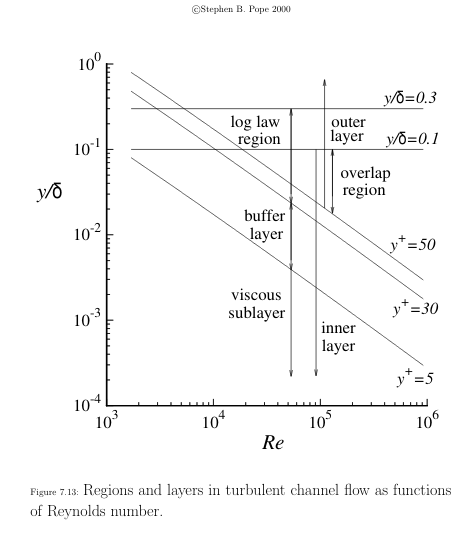 ] --- ## Mean velocity profiles In general (without any assumptions), on dimensional grounds, \\[ \frac{\partial \bar U}{\partial y} = \frac{u_*}{y} \Phi(y/\delta_v, y/\delta) \\] For \\( y / \delta \ll 1 \\), *tends asymptotically to* \\[ \frac{\partial \bar U}{\partial y} = \frac{u_*}{y} \Phi_1(y/\delta_v) \implies \frac{\partial u^+}{\partial y^+} = \frac{1}{y^+} \Phi_1(y^+) \\] ## Log-law of the wall von Karman (1930) postulated that for high \\( Re ,\, y / \delta \ll 1,\, y^+ \gg 1 \\), **negligible viscous effects**, which implies velocity profile is free from dependence of \\( \nu \\) or \\( y/\delta_v \\) \\[ \Phi_1 = \frac{1}{\kappa} \implies \frac{\partial u^+}{\partial y^+} = \frac{1}{\kappa y^+} \implies u^+ = \frac{1}{\kappa} \ln y^+ + B \\] --- ## Effect of roughness In general, the velocity gradient depends on 3 parameters. Including \\( s \\) the roughness scale: \\[ \frac{\partial \bar U}{\partial y} = \frac{u_*}{y} \Phi(y/\delta_v, y/\delta, s/\delta_v) \\] For the general case of roughtness size \\( s \sim \delta_v \\) we get, \\[ u^+ = \frac{1}{\kappa} \ln (y / s) + B(s / \delta_v) \\] other relations exist for extremes cases of small and large roughness scale \\( s \\). ## Note - The log-law is one among many established results in turbulence. - A similar approach is used in developing Monin-Obukhov similarity theory. --- class: center, middle, inverse # Monin-Obukhov similarity theory --- ## Governing parameters and assumptions Turbulence in the surface layer is determined by: 1. length scale \\( l \sim z \\) 1. velocity scale \\( u \sim u_* \\) 1. surface stress \\( \tau = \rho u_*^2 \\) 1. buoyancy parameter \\(\sim g/\theta_0 \\) 1. surface temperature flux \\( Q_0 \\) 1. ~~surface flux of a conserved scalar \\( C_0 \\)~~ ## Buckingham Pi theorem - \\( m = 5 \\) parameters - \\( n = 3 \\) dimensions: length, time, temperature, ~~scalar~~ implies the model can be rewritten using \\( m - n = 2 \\) independent dimensionless quantities. --- ## M-O functions .pull-left[ Similarity variable taken as \\( z/L \\), where *Monin-Obukhov length*: \\[ L = -u_*^3 \theta_0 / \kappa g Q_0 \\] 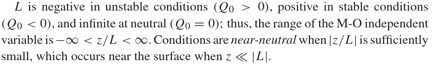 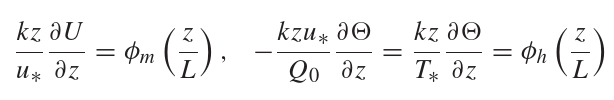 \\( L \\) being a function of the turbulence statistic \\( u_* \\) restricts a closed form solution of the M-O functions. These remained merely a theory until... ] .pull-right[ The 1968 Kansas experiment measured the LHS for different z and L and confirmed these functions are truly similar: 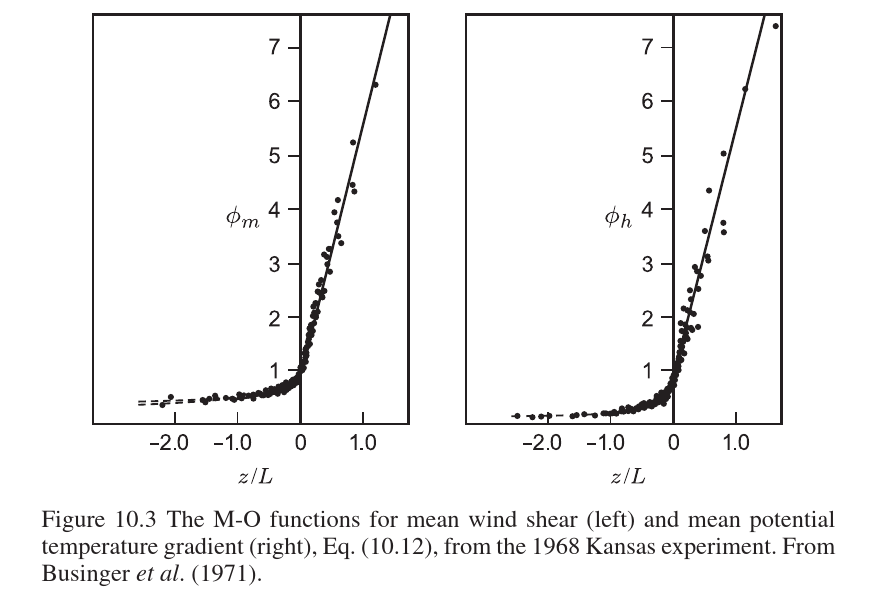 ] --- ## M-O functions and log-law In **neutral** conditions, \\( z/L \to 0 \implies \phi_m \approx 1\\) and we recover the classical log-law. \\[ \frac{\partial U}{\partial z} = \frac{u_*}{\kappa z} \\] \\[ U(z) = \frac{u_*}{\kappa} \left[ \ln z - \ln z_0 \right] \\] Compare the term \\( \ln z_0 \\) to roughness parameter \\(B\\). For **stable** and **unstable** regimes, curve fitting gives,  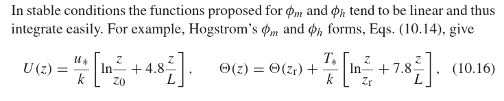 --- ## Moeng's variant .pull-left[ 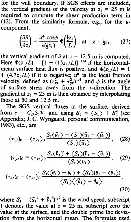 ] .pull-right[ #### Implementation in Nek5000 for neutral conditions \\[ \tau = \rho u_*^2 = \rho \left[ \frac{\kappa U}{\ln (z/z_0)}\right]^2 \\] which evaluated at \\( z = \frac{1}{2} z_1 \\) ```fortran ! --------Wall normal cordinate: `y` KAPPA = 0.41 y0 = 0.1 ! << y_max ! --------Calculate Moeng's model parameters ie = gllel(eg) u1_2 = (vx(ix,2,iz,ie) + vx(ix,1,iz,ie))/2 w1_2 = (vz(ix,2,iz,ie) + vz(ix,1,iz,ie))/2 absu = sqrt(u1_2**2 + w1_2**2) y1_2 = (ym1(ix,2,iz,ie) + ym1(ix,1,iz,ie))/2 ! --------Calculate Stresses trx = -KAPPA**2*(u1_2*absu)/(log(y1_2/y0)**2) try = 0.0 trz = -KAPPA**2*(w1_2*absu)/(log(y1_2/y0)**2) ``` ] --- .pull-left[ ## Physical aspects ### Meaning of \\( z/L \\) \\[ z / L = \frac{\text{buoyant production rate of turb. kinetic energy}}{\text{shear production rate of turb. kinetic energy}} \\] 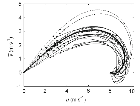 ] .pull-right[ ### Effect of boundary conditions - Average turning angle of the Ekmann spiral (bottom left) - Log-layer mismatch (bottom right) 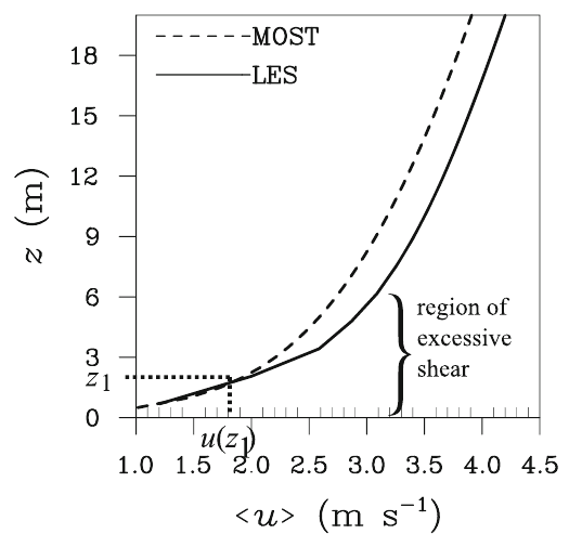 ] --- class: center, middle, inverse # Possible compressible formulation --- # Buoyancy frequency / stability .pull-left[ 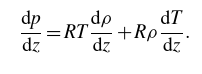 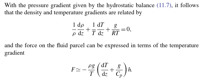 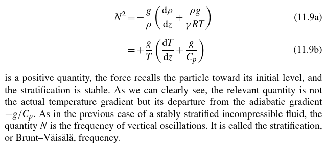 ] .pull-right[ 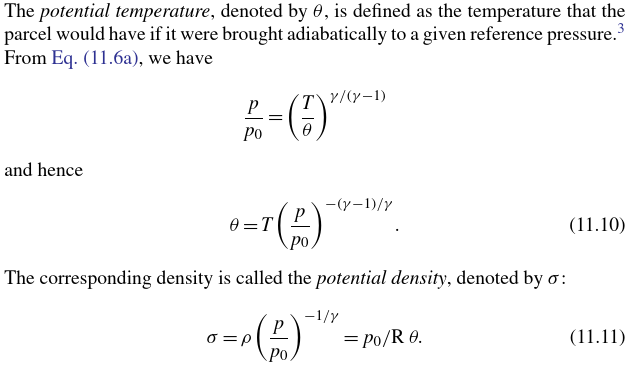 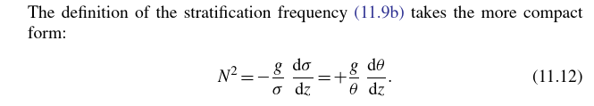 ] --- class: center, middle, inverse # Appendix: project update --- .pull-left[ # Filtering - Excessive filtering in last meeting - Filtering parameters were reduced - If time permits ... some visuals ] .pull-right[ # Next steps? Stay with neutral stratification - Oscillations - Sponge layer - Rayleigh radiative BC - Improved boundary condition: Robin conditions in literature - Comparison of statistics - Generated but unsure of what is plotted. - Need contact with a Ph.D. student using Nek5000. ] --- class: center, middle, inverse # Thank you for your attention! ### Any questions?  ## slides will be uploaded: [ashwin.info.tm/talks](https://ashwin.info.tm/talks.html)